 中级计量经济学第四章习题以及解答思路EViews.docx
- 文档编号:6101832
- 上传时间:2023-01-03
- 格式:DOCX
- 页数:21
- 大小:38.42KB
中级计量经济学第四章习题以及解答思路EViews.docx
《中级计量经济学第四章习题以及解答思路EViews.docx》由会员分享,可在线阅读,更多相关《中级计量经济学第四章习题以及解答思路EViews.docx(21页珍藏版)》请在冰豆网上搜索。
中级计量经济学第四章习题以及解答思路EViews
第4章
习题一
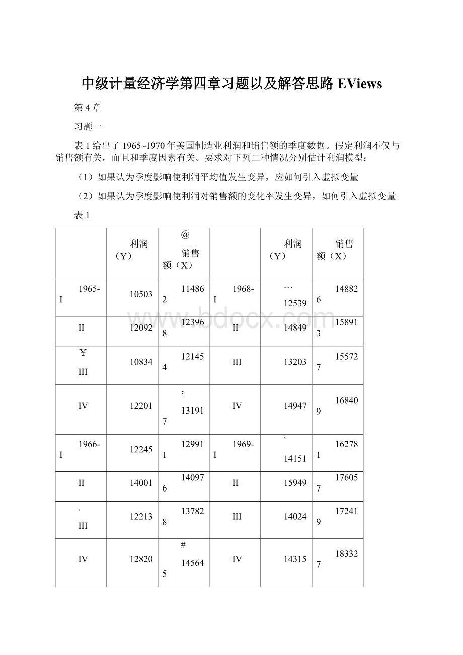
表1给出了1965~1970年美国制造业利润和销售额的季度数据。
假定利润不仅与销售额有关,而且和季度因素有关。
要求对下列二种情况分别估计利润模型:
(1)如果认为季度影响使利润平均值发生变异,应如何引入虚拟变量
(2)如果认为季度影响使利润对销售额的变化率发生变异,如何引入虚拟变量
表1
利润(Y)
@
销售额(X)
利润(Y)
销售额(X)
1965-I
10503
114862
1968-I
…
12539
148826
II
12092
123968
II
14849
158913
¥
III
10834
121454
III
13203
155727
IV
12201
;
131917
IV
14947
168409
1966-I
12245
129911
1969-I
`
14151
162781
II
14001
140976
II
15949
176057
.
III
12213
137828
III
14024
172419
IV
12820
#
145645
IV
14315
183327
1967-I
11349
136989
1970-I
'
12381
170415
II
12615
145126
II
13991
181313
¥
III
11014
141536
III
12174
176712
IV
12730
|
151776
IV
10985
180370
Quarterly65-70
Quick-EquationEstimation
[
Ycx@seas
(1)@seas
(2)@seas(3)
DependentVariable:
Y
Method:
LeastSquares
&
Date:
11/26/14Time:
18:
38
Sample:
1965Q11970Q4
Includedobservations:
24
$
【
Variable
Coefficient
Std.Error
t-Statistic
Prob.
}
"
C
X
"
@SEAS
(1)
-
@SEAS
(2)
@SEAS(3)
、
~
R-squared
Meandependentvar
、
AdjustedR-squared
.dependentvar
.ofregression
Akaikeinfocriterion
.
Sumsquaredresid
Schwarzcriterion
Loglikelihood
F-statistic
~
Durbin-Watsonstat
Prob(F-statistic)
/
T和P在5%情况下都不通过,第二季度相对还好一点
!
假设第二季度显著,结果的经济含义是什么
Ycx@seas
(2)@seas(3)@seas(4)
DependentVariable:
Y
Method:
LeastSquares
^
Date:
11/26/14Time:
18:
47
Sample:
1965Q11970Q4
;
Includedobservations:
24
%
Variable
Coefficient
Std.Error
,
t-Statistic
Prob.
'
C
:
X
@SEAS
(2)
@
@SEAS(3)
(
@SEAS(4)
;
R-squared
¥
Meandependentvar
AdjustedR-squared
.dependentvar
.ofregression
`
Akaikeinfocriterion
Sumsquaredresid
Schwarzcriterion
Loglikelihood
|
F-statistic
Durbin-Watsonstat
Prob(F-statistic)
@
"
第二季度依旧显著影响
四种都试一下(去掉一个季节),选一个最显著的
124
DependentVariable:
Y
Method:
LeastSquares
]
Date:
11/26/14Time:
18:
51
Sample:
1965Q11970Q4
(
Includedobservations:
24
"
Variable
Coefficient
Std.Error
{
t-Statistic
Prob.
?
C
、
X
@SEAS
(1)
>
@SEAS
(2)
{
@SEAS(4)
*
R-squared
$
Meandependentvar
AdjustedR-squared
.dependentvar
.ofregression
:
Akaikeinfocriterion
Sumsquaredresid
Schwarzcriterion
Loglikelihood
,
F-statistic
Durbin-Watsonstat
Prob(F-statistic)
#
&
134
DependentVariable:
Y
Method:
LeastSquares
.
Date:
11/26/14Time:
18:
52
Sample:
1965Q11970Q4
Includedobservations:
24
—
Variable
Coefficient
Std.Error
t-Statistic
Prob.
\
>
C
X
】
@SEAS
(1)
·
@SEAS(3)
@SEAS(4)
?
'
R-squared
Meandependentvar
…
AdjustedR-squared
.dependentvar
.ofregression
Akaikeinfocriterion
·
Sumsquaredresid
Schwarzcriterion
Loglikelihood
F-statistic
*
Durbin-Watsonstat
Prob(F-statistic)
(
(2)
}
Y=c+βx+α1D1X+α2D2X+α3D3X
D1=1(第一季度)0(其他)
Ycx@seas
(1)*x@seas
(2)*x@seas(3)*x
DependentVariable:
Y
Method:
LeastSquares
~
Date:
11/26/14Time:
19:
00
Sample:
1965Q11970Q4
、
Includedobservations:
24
]
Variable
Coefficient
Std.Error
。
t-Statistic
Prob.
《
C
@
X
@SEAS
(1)*X
》
@SEAS
(2)*X
(
@SEAS(3)*X
:
R-squared
`
Meandependentvar
AdjustedR-squared
.dependentvar
.ofregression
;
Akaikeinfocriterion
Sumsquaredresid
Schwarzcriterion
Loglikelihood
.
F-statistic
Durbin-Watsonstat
Prob(F-statistic)
:
)
DependentVariable:
Y
Method:
LeastSquares
?
Date:
11/26/14Time:
19:
10
Sample:
1965Q11970Q4
Includedobservations:
24
·
$
Variable
Coefficient
Std.Error
t-Statistic
Prob.
|
;
C
X
/
@SEAS
(1)
:
@SEAS(3)
@SEAS(4)
|
(
R-squared
Meandependentvar
《
AdjustedR-squared
.dependentvar
.ofregression
Akaikeinfocriterion
^
Sumsquaredresid
Schwarzcriterion
Loglikelihood
F-statistic
%
Durbin-Watsonstat
Prob(F-statistic)
—
@
DependentVariable:
Y
Method:
LeastSquares
Date:
11/26/14Time:
19:
11
:
Sample:
1965Q11970Q4
Includedobservations:
24
…
'
Variable
Coefficient
Std.Error
t-Statistic
Prob.
|
¥
C
X
/
@SEAS
(1)*X
@SEAS
(2)*X
(
@SEAS(4)*X
"
、
R-squared
Meandependentvar
AdjustedR-squared
{
.dependentvar
.ofregression
Akaikeinfocriterion
Sumsquaredresid
【
Schwarzcriterion
Loglikelihood
F-statistic
Durbin-Watsonstat
/
Prob(F-statistic)
'
DependentVariable:
Y
、
Method:
LeastSquares
Date:
11/26/14Time:
19:
11
Sample:
1965Q11970Q4
|
Includedobservations:
24
】
Variable
…
Coefficient
Std.Error
t-Statistic
Prob.
}
C
~
X
]
@SEAS
(2)*X
@SEAS(3)*X
(
@SEAS(4)*X
>
/
R-squared
Meandependentvar
AdjustedR-squared
.dependentvar
)
.ofregression
Akaikeinfocriterion
Sumsquaredresid
Schwarzcriterion
"
Loglikelihood
F-statistic
Durbin-Watsonstat
Prob(F-statistic)
*
¥
习题二
表2给出了某地区某行业的库存
和销售
的统计资料。
假设库存额依赖于本年销售额与前三年的销售额,试用Almon变换估计以下有限分布滞后模型:
`
表2
库存Y
(万元)
销售额X
(万元)
库存Y
》
(万元)
销售额X
(万元)
1980
11267
8827
1990
17053
{
13668
1981
12661
9247
1991
19491
14956
1982
:
12968
9579
1992
21164
15483
1983
12518
9093
"
1993
22719
16761
1984
13177
10073
1994
24269
·
17852
1985
13454
10265
1995
25411
17620
1986
!
13735
10299
1996
25611
18639
1987
14553
11038
>
1997
26930
20672
1988
15011
11677
1998
30218
·
23799
1989
15846
12445
1999
36784
27359
]
Y=α+α0ΣXt-i+α1ΣXt-i+α2ΣXt-i+μt
↑3,i=0笔记11,26)
在最上面输入
genrz0=x+x(-1)+x(-1)+x(-3)
genrz1=x(-1)+2*x(-2)+3*x(-3)
genrz2=x(-1)+4*x(-2)+9*x(-3)
.
ycz0z1z2
DependentVariable:
Y
Method:
LeastSquares
?
Date:
11/26/14Time:
19:
38
Sample(adjusted):
19831999
Includedobservations:
17afteradjustments
(
(
Variable
Coefficient
Std.Error
t-Statistic
Prob.
】
、
C
Z0
?
Z1
|
Z2
;
*
R-squared
Meandependentvar
AdjustedR-squared
.dependentvar
。
.ofregression
Akaikeinfocriterion
Sumsquaredresid
2692398.
Schwarzcriterion
-
Loglikelihood
F-statistic
Durbin-Watsonstat
Prob(F-statistic)
】
《
YcPDL(x,3,2)
重新回归
DependentVariable:
Y
'
Method:
LeastSquares
Date:
11/26/14Time:
19:
46
Sample(adjusted):
19831999
~
Includedobservations:
17afteradjustments
…
"
Variable
Coefficient
Std.Error
t-Statistic
Prob.
~
—
C
"
PDL01
PDL02
)
PDL03
"
&
R-squared
:
Meandependentvar
AdjustedR-squared
.dependentvar
&
.ofregression
Akaikeinfocriterion
Sumsquaredresid
2511848.
?
Schwarzcriterion
Loglikelihood
F-statistic
Durbin-Watsonstat
;
Prob(F-statistic)
|
LagDistributionofX
i
Coefficient
Std.Error
t-Statistic
、
;
.*|
0
{
.*|
1
.*|
}
2
*.|
3
>
^
SumofLags
-
》
'
习题三
表3给出了印度1949~1965年实际货币存量、实际总国民收入和长期利率数据。
假设有如下的长期货币需求关系式:
其中,
为长期货币需求(现金余额);
为长期利率;
为实际总国民收入。
请在如下存量调整假说下估计该货币需求模型,其中
为实际现金存量:
表3
…
年份
实际
货币M
实际
净收入Y
长期
利率R
年份
)
实际
货币M
实际
净收入Y
长期
利率R
(千万卢比)
、
(10亿卢比)
(%)
(千万卢比)
(10亿卢比)
(%)
1949
(
1958
1950
&
1959
1951
[
1960
1952
>
1961
1953
$
1962
1954
]
1963
1955
;
1964
1956
'
1965
1957
)
LnM*t=lnβ0+β1lnRt+β2lnYt+μt
~
LnMt-LnMt-1=
lnM*t-
lnMt-1
LnMt=
lnβ0+β1
lnRt+β2
lnYt+(1-
)lnMt-1+
μt
求回归
Quick-EquationEstimation
log(m)clog(r)log(y)log(m(-))
DependentVariable:
LOG(M)
/
Method:
LeastSquares
Date:
11/26/14Time:
20:
13
Sample(adjusted):
19501965
;
Includedobservations:
16afteradjustments
;
Variable
Coefficient
》
Std.Error
t-Statistic
Prob.
!
C
!
LOG(R)
LOG(Y)
$
LOG(M(-1))
《
R-squared
Meandependentvar
AdjustedR-squared
.dependentvar
.ofregre


- 配套讲稿:
如PPT文件的首页显示word图标,表示该PPT已包含配套word讲稿。双击word图标可打开word文档。
- 特殊限制:
部分文档作品中含有的国旗、国徽等图片,仅作为作品整体效果示例展示,禁止商用。设计者仅对作品中独创性部分享有著作权。
- 关 键 词:
- 中级 计量 经济学 第四 习题 以及 解答 思路 EViews
 冰豆网所有资源均是用户自行上传分享,仅供网友学习交流,未经上传用户书面授权,请勿作他用。
 铝散热器项目年度预算报告.docx
-
牛津上海版通用小学英语三年级上册Unit 12同步练习2II 卷.docx
-
论我国私营企业员工激励机制.docx
-
人教版五年级品德与社会上册全册教案.docx
-
开学啦国旗下讲话稿三分钟.docx
-
露天采矿学复习题.docx
-
六年级英语教师年度考核个人总结.docx
-
某路站综合体项PC吊装施工方案.docx
-
人教版九年级历史上册期末考试试题一套.docx
-
隆昌妇幼保健院.docx
-
芦二矿抽采达标中长期规划.docx
-
看拼音写词语.docx
-
模拟磁盘调度算法系统的设计毕业设计.docx
-
每周一条名言警句或一首诗词.docx
-
棉花膜下滴灌示范工程设计总结报告.docx
-
九年级化学教案第十单元酸和碱教案新人教版.docx
-
宁波市水资源公报.docx
-
农业实用技术培训工作意见与农业局上半年工作总结范例两篇汇编.docx
-
平行线的判定.docx
-
内部会计管理制度11成本核算制度.docx
-
盘扣式脚手架支撑方案.docx
-
旅游规划模板.docx
-
煤矿大本大专毕业设计大采高综采工作面作业规程.docx
-
美学选择题整理课件资料.docx
-
名家论腹泻慢性肠炎.docx
-
宁夏银川市第一中学学年高一上学期期中考试地理试题解析解析版.docx
-
年产吨精密纤维纸项目建设建议书.docx
-
农技推广中心工作总结.docx
-
彭宇案的法逻辑批判.docx
-
宁夏仕奇房产网发布份房地产交易情况.docx
-
项目推荐书智能温控节能系统.docx
-
区县节日期间加强消防安全讲话稿与区发改委领导班子述职述廉报告汇编.docx
-
数据中心机房设计建设方案.docx
-
数字图像处理MATLAB相关代码.docx
-
水夯法基坑回填方案.docx
-
水上乐园项目申请报告讲解.docx
-
司发53号安全禁令.docx
-
四川省广安市邻水县学年高二物理下学期第一次月考试题20含答案.docx
-
四六级常考词组一#####.docx
-
四年级数学教学工作总结范文.docx
-
饲料实习报告.docx
-
苏教版小学六年级上册《水滴里的生物》PPT课件之一综述.docx
-
塑料模具成型部分设计.docx
-
台州美丽田园综合体创建导则.docx
-
唐七公子著作经典爱情语录.docx
-
特斯拉专利解析报告.docx
-
体育艺术2+1项目实施方案设计.docx
-
天津武清区学年高二上学期期中考试语文试题扫描版.docx
-
跳绳比赛活动策划方案.docx
-
停车场应急预案三篇doc.docx
-
生物与环境生态系统.docx
