 DSP数字信号处理实验Matlab实验代码及输出图.docx
- 文档编号:2384018
- 上传时间:2022-10-29
- 格式:DOCX
- 页数:21
- 大小:349.54KB
DSP数字信号处理实验Matlab实验代码及输出图.docx
《DSP数字信号处理实验Matlab实验代码及输出图.docx》由会员分享,可在线阅读,更多相关《DSP数字信号处理实验Matlab实验代码及输出图.docx(21页珍藏版)》请在冰豆网上搜索。
DSP数字信号处理实验Matlab实验代码及输出图
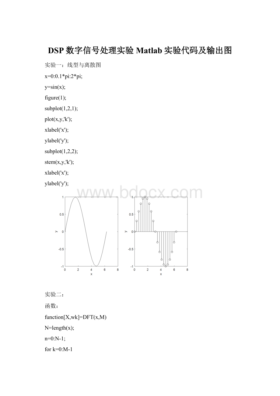
实验一:
线型与离散图
x=0:
0.1*pi:
2*pi;
y=sin(x);
figure
(1);
subplot(1,2,1);
plot(x,y,'k');
xlabel('x');
ylabel('y');
subplot(1,2,2);
stem(x,y,'k');
xlabel('x');
ylabel('y');
实验二:
函数:
function[X,wk]=DFT(x,M)
N=length(x);
n=0:
N-1;
fork=0:
M-1
wk(k+1)=2*pi/M*k;
X(k+1)=sum(x.*exp(-j*wk(k+1)*n));
end
clc;
clearall;
A=444.128;
a=50*sqrt
(2)*pi;
w0=50*sqrt
(2)*pi;
fs=input('输入采样频率fs=');
T=1/fs;
N=50;
n=0:
N-1;
xa=A*exp(-a*n*T).*sin(w0*n*T);
subplot(1,2,1);
stem(n,xa,'.');
grid;
M=100;
[Xa,wk]=DFT(xa,M);
f=wk*fs/(2*pi);
subplot(1,2,2);
plot(f,abs(Xa));
grid;
1000hz
500hz
200hz
DFT程序:
Clc
clearall
xbn=[1,0,0,0];
hbn=[1,2.5,2.5,1]
N=4;
n=0:
N-1;
Xb=fft(xbn,N);
Xh=fft(hbn,N);
ybn=conv(xbn,hbn);
subplot(3,2,1);
stem(n,xbn,'.');
title('xbnwave');
subplot(3,2,2);
stem(n,abs(Xb),'.');
title('Xbwave');
subplot(3,2,3);
stem(n,hbn,'.');
title('hbnwave');
subplot(3,2,4);
stem(n,abs(Xh),'.');
title('Xhwave');
n1=0:
6;
Xy=fft(ybn,8);
subplot(3,2,5);
stem(n1,ybn,'.');
title('ybnwave')
n2=0:
7;
subplot(3,2,6);
stem(n2,abs(Xy),'.');
title('Xywave
结果:
hbn=
1.00002.50002.50001.0000
实验三:
第一个方程:
clc;
clearall;
a1=[1,0.75,0.125];
b1=[1,-1];
n=0:
20;
x1=[1zeros(1,20)];
subplot(2,3,1);
y1filter=filter(b1,a1,x1);
stem(n,y1filter);
title('ylfilter');
xlabel('x');
ylabel('y');
x1=[1zeros(1,10)];
[h]=impz(b1,a1,10);
subplot(2,3,2);
y1conv=conv(h,x1);
n=0:
19;
stem(n,y1conv,'filled')
subplot(2,3,3);
impz(b1,a1,21);
n=0:
20;
x2=ones(1,21);
subplot(2,3,4);
y1filter=filter(b1,a1,x2);
stem(n,y1filter);
title('y1filter_step');
xlabel('x');
ylabel('y');
x2=ones(1,21);
[h]=impz(b1,a1,20);
y1=conv(h,x2);
y1conv=y1(1:
21);
n1=0:
20;
subplot(2,3,5);
stem(n1,y1conv,'filled');
title('y1conv');
xlabel('n');
ylabel('y1[n]');
subplot(2,3,6);
b1=1;
impz(b1,a1);
第二个方程:
clc;
clearall;
a1=[1];
b1=[0.25,0.25,0.25,0.25];
n=0:
20;
x1=[1zeros(1,20)];
y1filter=filter(b1,a1,x1);
subplot(2,3,1);
stem(n,y1filter);
title('y1filter');
xlabel('x');
ylabel('y');
x1=[1zeros(1,10)];
[h]=impz(b1,a1,10);
y1conv=conv(h,x1);
n=0:
19;
subplot(2,3,2);
stem(n,y1conv,'filled')
subplot(2,3,3);
impz(b1,a1,21);
n=0:
20;
x2=ones(1,21);
y1filter=filter(b1,a1,x2);
subplot(2,3,4);
stem(n,y1filter);
title('y1filter_step');
xlabel('x');
ylabel('y');
x2=ones(1,21);
[h]=impz(b1,a1,20);
y1=conv(h,x2);
y1conv=y1(1:
21);
n1=0:
20;
subplot(2,3,5);
stem(n1,y1conv,'filled');
title('y1conv');
xlabel('n');
ylabel('y1[n]');
subplot(2,3,6);
n=0:
20;
a1=1;
b1=[0,0.25,0.5,0.75,ones(1,17)];
impz(b1,a1,21);
第一个方程结果
第二个方程结果:
实验四:
程序:
clc;
clearall;
num=[0.05280.07970.12950.12950.7970.0528];
den=[1-1.81072.4947-1.88010.9537-0.2336];
[z,p,k]=tf2zp(num,den);
m=abs(p);
disp('零点');disp(z);
disp('极点');disp(p);
disp('增益系数');disp(k);
sos=zp2sos(z,p,k);
figure
(1)
subplot(2,3,5);
zplane(num,den)
k=256;
w=0:
pi/k:
pi;
h=freqz(num,den,w);
subplot(2,3,1);
plot(w/pi,real(h));grid
title('实部')
xlabel('\omega/\pi');ylabel('幅度')
subplot(2,3,2);
plot(w/pi,imag(h));grid
title('虚部')
xlabel('\omega/\pi');ylabel('Amplitude')
subplot(2,3,3);
plot(w/pi,abs(h));grid
title('幅度谱')
xlabel('\omega/\pi');ylabel('幅值')
subplot(2,3,4);
plot(w/pi,angle(h));grid
title('相位谱')
xlabel('\omega/\pi');ylabel('弧度')
figure
(2)
freqz(num,den,128);
结果:
零点
-1.5870+1.4470i
-1.5870-1.4470i
0.8657+1.5779i
0.8657-1.5779i
-0.0669+0.0000i
极点
0.2788+0.8973i
0.2788-0.8973i
0.3811+0.6274i
0.3811-0.6274i
0.4910+0.0000i
增益系数
0.0528
实验五:
clc;clearall;
wp=input('通带内频率wp=');
ap=input('容许幅度误差ap=');
ws=input('频率ws=');
as=input('阻带衰减as=');
fs=1;
[N,Wn]=buttord(wp,ws,ap,as,'s');
[Z,P,K]=buttap(N);
[Bap,Aap]=zp2tf(Z,P,K);
[b,a]=lp2lp(Bap,Aap,Wn);
[bz,az]=bilinear(b,a,fs);
[H,W]=freqz(bz,az,64);
subplot(2,1,1);
stem(W/pi,abs(H));
grid;
xlabel('频率');
ylabel('幅度');
subplot(2,1,2);
stem(W/pi,20*log10(abs(H)));
grid;
xlabel('频率');
ylabel('幅度(dB)');
bz
az
结果:
通带内频率wp=0.1*pi
容许幅度误差ap=0.5
频率ws=0.5*pi
阻带衰减as=20
bz=
0.02380.07140.07140.0238
az=
1.0000-1.62171.0505-0.2384
实验六:
Blackman方式:
clc;
clearall;
b=fir1(21,0.5,blackman(22));
figure
(1);
y=freqz(b,1);
subplot(2,2,1);
plot(abs(y));
grid;
title('幅度响应');
subplot(2,2,2);
plot(angle(y));
grid;
title('相位响应');
subplot(2,2,3);
cj=impz(b,1,20);
stem(cj);
title('冲激响应');
grid;
Hamming方式:
clc;
clearall;
b=fir1(21,0.5,hamming(22));
figure
(1);
y=freqz(b,1);
subplot(2,2,1);
plot(abs(y));
grid;
title('幅度响应');
subplot(2,2,2);
plot(angle(y));
grid;
title('相位响应');
subplot(2,2,3);
cj=impz(b,1,20);
stem(cj);
title('冲激响应');
grid;
Hanning方式:
clc;
clearall;
b=fir1(21,0.5,hanning(22));
figure
(1);
y=freqz(b,1);
subplot(2,2,1);
plot(abs(y));
grid;
title('幅度响应');
subplot(2,2,2);
plot(angle(y));
grid;
title('相位响应');
subplot(2,2,3);
cj=i


- 配套讲稿:
如PPT文件的首页显示word图标,表示该PPT已包含配套word讲稿。双击word图标可打开word文档。
- 特殊限制:
部分文档作品中含有的国旗、国徽等图片,仅作为作品整体效果示例展示,禁止商用。设计者仅对作品中独创性部分享有著作权。
- 关 键 词:
- DSP 数字信号 处理 实验 Matlab 代码 输出
 冰豆网所有资源均是用户自行上传分享,仅供网友学习交流,未经上传用户书面授权,请勿作他用。
 转基因粮食的危害资料摘编Word下载.docx
-
高中英语词组大全Word文档下载推荐.docx
-
卫计局年工作总结及新年工作计划Word格式.docx
-
贵州省煤矿安全管理人员安全资格证A考试概况Word格式.docx
-
系统集成项目招标文件Word文件下载.docx
-
消防设计技术审查的要点Word文档格式.docx
-
第三章 习题课 带电粒子在磁场或复合场中的运动Word格式.docx
-
湖南岳阳中考英语模拟卷含答案Word文档格式.docx
-
电子商务考试题总汇打印版打印打印Word下载.docx
-
选调生考试备考言语理解与表达真题Word文档格式.docx
-
高考物理实验题专练 专练15Word文档格式.docx
-
加装奥迪A4L蓝牙电话功能Word文档下载推荐.docx
-
学年下学期好教育高三月考仿真卷A卷 语文 学生版后附详解Word文档下载推荐.docx
-
净化生产车间工程一般施工技术施工方案Word文档格式.docx
-
内蒙古呼和浩特市第六中学学年高一政治下学期期末考试试题Word下载.docx
-
证券行业客户经理电话营销技巧与实例Word文档下载推荐.docx
-
叶芝 苇间风文档格式.docx
-
最新中美贸易摩擦的原因及解决对策1论文Word文件下载.docx
-
意义的近义词Word格式文档下载.docx
-
上海市中考英语试题S.docx
-
专题12观点论证类设问.docx
-
附加安心重疾条款.docx
-
设计变更管理办法修改意见稿FINAL汇编.docx
-
毕业赠言毕业致词精选多篇.docx
-
银行新员工代表发言稿精选多篇.docx
-
北京市朝阳区届高三第一学期期末语文试题Word版含答案.docx
-
HL线切割使用说明书模板.docx
-
车工实训周记.docx
-
USBHID键盘扫描码.docx
-
Apmpoqu4调研报告.docx
-
最熟悉的陌生人作文八篇.docx
-
被动语态综合讲解.docx
-
探索农村金融改革新思路1.docx
-
世界大学城空间美化代码.docx
-
土方工程承包协议书范本.docx
-
完整版中级会计职称财务管理知识点归纳总结.docx
-
数学建模习题.docx
-
混凝土结构设计原理复习重点非常好讲课教案.docx
-
全新版大学英语第二版综合教程2最全的课后练习答案.docx
-
牙克石商业会所设计感悟.docx
-
监控设计方案.docx
-
一盏一盏的灯读后感.docx
-
施工班组目标工作责任书.docx
-
高二地理联考试题.docx
-
全自动洗衣机毕业设计及组态王仿真.docx
-
四年级数学上册口算基础99.docx
-
监守自盗观后感.docx
-
毕业设计曹妃甸油气田群安全评价报告.docx
-
介词与某些词类的搭配.docx
-
学生会期末工作总结模板4篇.docx
-
少先队辅导员工作总结4篇.docx
