 MATLAB实验代码.docx
- 文档编号:28241584
- 上传时间:2023-07-09
- 格式:DOCX
- 页数:10
- 大小:35.67KB
MATLAB实验代码.docx
《MATLAB实验代码.docx》由会员分享,可在线阅读,更多相关《MATLAB实验代码.docx(10页珍藏版)》请在冰豆网上搜索。
MATLAB实验代码
实验1
1、ones语句:
Y=ones(n)%生成n×n全1阵
Y=ones(m,n)%生成m×n全1阵
Y=ones([mn])%生成m×n全1阵
Y=ones(d1,d2,d3…)%生成d1×d2×d3×…全1阵或数组
Y=ones([d1d2d3…])%生成d1×d2×d3×…全1阵或数组
Y=ones(size(A))%生成与矩阵A相同大小的全1阵
2、find语句:
k=find(x)%按行检索X中非零元素的点,若没有非零元素,将返回空矩阵。
[i,j]=find(X)%检索X中非零元素的行标i和列标j。
[i,j,v]=find(X)%检索X中非零元素的行标i和列标j以及对应的元素值v。
实验3
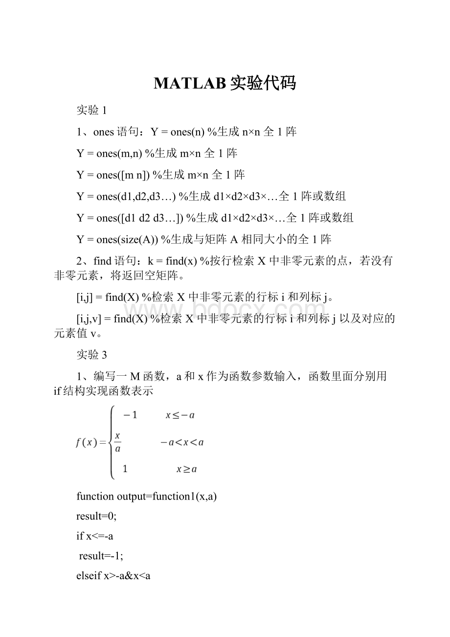
1、编写一M函数,a和x作为函数参数输入,函数里面分别用if结构实现函数表示
functionoutput=function1(x,a)
result=0;
ifx<=-a
result=-1;
elseifx>-a&x result=x/a; elsex>=a result=1; end output=[result]; 2、编写一M函数,迭代计算 ,给出可能的收敛值,其中x的初值作为函数的参数输入。 functionoutput=function2(x) y=0; while1 y=3/(x+2); ifabs(y-x)<0.000001 break; elsex=y; end end output=[y]; end 3、编写一M函数,实现 近似计算指数,其中x为函数参数输入,当n+1步与n步的结果误差小于0.00001时停止,分别用for和while结构实现。 用for结构实现: functionoutput=function3(x) e=0;s=0;i=0; while1 e=s+x^i/factorial(i); ifabs(e-s)<0.000001 break; elses=e;i=i+1; end end output=[e]; 用while结构实现: functionoutput=function4(x) s=1;e=0; fori=1: 1000000 e=s+x^i/factorial(i); ifabs(e-s)<0.00001 break; elses=e; end end output=[e]; 实验4 1.绘制函数 的曲线,其中曲线为绿虚线,并进行标注 x=-2: 0.1: 1; y=x.^2; plot(x,y,'--g'); holdon x=1: 0.1: 2; y=exp(-(x-1).^2); plot(x,y,'--g') text(-1,1,'曲线y1=x^2'); text(1.5,0.5,'曲线y1=e^(-(x-1)^2)'); 2.将用于绘制曲线 的数据分别保存成MAT、二进制的文本文件中 t=[0: pi/10: 2*pi]; x=[sin(t)sin(t)]; y=[cos(t)cos(t)]; z=[sin(t).*cos(t)]; savemydatafilexyz clear loadmydatafile d=z t=[0: pi/10: 2*pi]; x=[sin(t)]; y=[cos(t)]; z=[sin(t).*cos(t)]; fid=fopen('text.txt','w') count=fwrite(fid,z,'float32') closestatus=fclose(fid) 3.重启Matlab,从上述保存的文件中依次读取变量z的前10个数据 fid=fopen('mydatafile.mat','r') data1=fread(fid,10) fid=fopen('text.txt','r'); data2=fread(fid,10) 实验5 1.将多项式A的系数向量形式[13631]转换为完整形式,并求其根。 同时在0-5内随机产生150组自变量,计算他们的对应取值; A=[13631]; [s,len]=poly2str(A,'x') 求根: r=roots(A) 产生0-5内150组自变量: q=5*rand(1,150) 计算对应取值: w=polyval(A,q) 2.对于上述150组数据,采用多项式进行拟合,并对 分别采用最邻近、双线性和三次样条插值方法进行插值; x=1: 4; y=x.^4+3.*x.^3+6.*x.^2+3.*x+1; xi=1: 0.1: 10; yi_nearest=interp1(x,y,xi,'nearset'); yi_linear=interp1(x,y,xi); yi_spline=interp1(x,y,xi,'spline'); figure; holdon; subplot(1,3,1); plot(x,y,'ro',xi,yi_nearest,'b-'); title('最邻近插值'); subplot(1,3,2); plot(x,y,'ro',xi,yi_linear,'b-'); title('线性插值'); subplot(1,3,3); plot(x,y,'ro',xi,yi_spline,'b-'); title('三次样条插值'); 3、计算 symsxy t=int(y*exp(x),y,2*y) int(t,1,2) 实验6 1、连续信号的产生与可视化,直流信号、正弦交流信号、单位阶跃信号、单位冲击信号、符号信号、斜坡信号、单位衰减信号、复指数信号等实现以及可视化 直流信号: x1=[-5: 0.01: 0]; y1=1; plot(x1,y1); holdon x2=[0: 0.01: 5]; y2=1; plot(x2,y2) 正弦交流信号: x=[0: 0.01: 2*pi]; y=sin(x); plot(x,y) 单位阶跃信号: t=-4: 0.01: 4; f=(t>0); stairs(t,f); axis([-4,4,-1.1,1.1]); 单位冲击信号: t=-4: 0.01: 4; n=length(t); f=zeros(1,n); f(1,(-t0+4)/0.01+1)=1; plot(t,f); axis([-4,4,-1.1,1.1]); 符号信号: t=-4: 0.01: 4; f=sign(t); plot(t,f); axis([-4,4,-1.1,1.1]); 斜坡信号: t=0: 0.01: 4; f=t; plot(t,f); axis([0,4,0,4]); 单位衰减信号: t=0: 0.01: 10; y=10*exp(-10*t).*sin(10*t); plot(t,y); 复指数信号: t=-10: 0.1: 10; y=exp(10+j*t); plot(t,y); 2、将信号 与信号 进行加、减、乘运算,并且将结果可视化。 加法运算: t=-10: 0.1: 10; y=exp(-3*t)+0.2*sin(4*pi*t); plot(t,y); 减法运算: t=-10: 0.1: 10; y=exp(-3*t)-0.2*sin(4*pi*t); plot(t,y); 乘法运算: t=-10: 0.1: 10; y=(exp(-3*t)).*(0.2*sin(4*pi*t)); plot(t,y); 3已知信号 ,试通过反褶、移位、尺度变换由 的波形得到 的波形。 定义符号函数f(t)=sin(t)/t: symst; f=sym('sin(t)/t'); 对f进行移位: f1=subs(f,t,t+3); 对f1进行尺度变换: f2=subs(f1,t,2*t); 对f2进行反褶: f3=subs(f2,t,-t); 绘制函数波形: subplot(2,2,1);ezplot(f,[-8,8]);gridon; subplot(2,2,2);ezplot(f1,[-8,8]);gridon; subplot(2,2,3);ezplot(f2,[-8,8]);gridon; subplot(2,2,4);ezplot(f3,[-8,8]);gridon; 4、分别产生两个方波信号,并且求这两个方波的卷积。 产生两个方波: y1=[ones(1,10),zeros(1,20)]; y2=[ones(1,30),zeros(1,20)]; 两个方波卷积: y=conv(y1,y2); n1=1: length(y1); n2=1: length(y2); L=length(y); n=1: L; %显示波形: subplot(3,1,1);plot(n1,y1);axis([1,L,0,2]); subplot(3,1,2);plot(n2,y2);axis([1,L,0,2]); subplot(3,1,3);plot(n,y);axis([1,L,0,20]);


- 配套讲稿:
如PPT文件的首页显示word图标,表示该PPT已包含配套word讲稿。双击word图标可打开word文档。
- 特殊限制:
部分文档作品中含有的国旗、国徽等图片,仅作为作品整体效果示例展示,禁止商用。设计者仅对作品中独创性部分享有著作权。
- 关 键 词:
- MATLAB 实验 代码
 冰豆网所有资源均是用户自行上传分享,仅供网友学习交流,未经上传用户书面授权,请勿作他用。
 《贝的故事》教案4.docx
-
《对韵歌》优秀教案8.docx
-
《函数yAsinωx+φ+P图象》wwwnet.docx
-
《静夜思》教学设计.docx
-
《汽车底盘构造与维修》题库与考核标准.docx
-
《世说新语》复习资料.docx
-
《我的服装我做主》教案设计.docx
-
《在品味情感中成长》教学片断设计.docx
-
11造价员《建设工程造价管理基础知识》精讲教程文件.docx
-
《不会叫的狗》教案 人教部编版1.docx
-
《操作系统》二学期A卷及答案.docx
-
《傅雷家书》名著阅读笔记.docx
-
《反不正当竞争法》下互联网平台封禁行为考辨以消费者用户合法权益保护为中心.docx
-
《化工原理》第六章蒸发.docx
-
《蓝海战略》概要11页.docx
-
《人生》读书心得.docx
-
《荷叶圆圆》公开课教案优秀教学设计26.docx
-
《科技出行研究报告》智能网联与新能源将变革未来汽车出行.docx
-
《272 向量的应用举例》导学案1.docx
-
《秋天》评课稿.docx
-
《电算化》第二章会计电算化的工作环境章节练习.docx
-
《室外给排水管道》施组.docx
-
《广东省建筑与装饰工程综合定额》计算规则.docx
-
《我多想去看看》教学.docx
-
《直通车车手基础认证》 考试答案 70题之欧阳育创编.docx
-
7天销量翻10倍皇冠卖家教您玩转最精准流量.docx
-
9 阿长和山海经.docx
-
《比例尺》教案.docx
-
《菜根谭》注译四闲适篇.docx
-
《福尔摩斯探案集》读后感15篇.docx
-
《红对勾》古代诗歌选择题答案补充.docx
-
《课堂密码》读后感及心得精选多篇.docx
-
竞争法 刘继峰.docx
-
公路试验检测频率一览表Word格式.docx
-
广西百色市学年高一下学期期末考试英语试题Word文件下载.docx
-
国家空气监测城市站运行管理规定文档格式.docx
-
金融市场学章节练习题及答案01共12章.docx
-
32个管理学经典理论Word格式文档下载.docx
-
关于幼儿园开学自查报告范文经典五篇精选文档格式.docx
-
宏观经济因素对房价的影响Word下载.docx
-
《反义词》大班教案Word文档下载推荐.docx
-
工业分析与分离复习资料Word文档格式.docx
-
购货基本合同Word文件下载.docx
-
国内标杆地产人力资源 内部讲师评选方案Word文件下载.docx
-
病房医生站使用说明书文档格式.docx
-
广州图书馆法人治理结构试点概况教程文件Word格式文档下载.docx
-
国有土地使用权出让合同范本新版Word文档格式.docx
-
护理实习报告范文2篇Word格式文档下载.docx
-
光伏发电采购合同范本Word格式.docx
-
关于努力学习的作文通用25篇文档格式.docx
-
国有土地使用权出让协议标准范本Word下载.docx
